
Preface
Many data pipeline frameworks offer very similar functionality. With this in mind, Google developed a unified data pipeline framework under the name Cloud Dataflow SDK. This framework was later donated to the Apache Software Foundation. It was then named Apache Beam. Let’s look at the following figure to understand Apache Beam better.
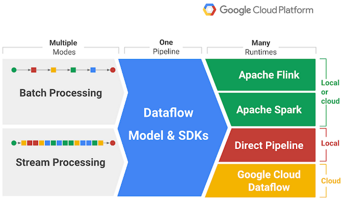
We create a single pipeline, which then allows us to do either Batch Processing or Stream Processing. The processing is realized with a Runtime of our choice. We can test our code locally with Direct Pipeline or send it to a cloud service such as Google Cloud Dataflow. This makes Apache Beam a very interesting framework to try.
In this article, we will analyze a COVID dataset with Apache Beam.
The Dataset
The dataset is in the german language, but don’t worry, I will explain the relevant parts. The dataset is provided by the Robert-Koch-Institut here. The dataset looks as follows.
FID,IdBundesland,Bundesland,Landkreis,Altersgruppe,Geschlecht,AnzahlFall,AnzahlTodesfall,Meldedatum,IdLandkreis,Datenstand,NeuerFall,NeuerTodesfall,Refdatum,NeuGenesen,AnzahlGenesen,IstErkrankungsbeginn,Altersgruppe2
1,1,Schleswig-Holstein,SK Kiel,A15-A34,M,1,0,2020/03/23 00:00:00,01002,"15.12.2020, 00:00 Uhr",0,-9,2020/03/20 00:00:00,0,1,1,Nicht übermittelt
2,1,Schleswig-Holstein,SK Flensburg,A00-A04,M,1,0,2020/09/30 00:00:00,01001,"15.12.2020, 00:00 Uhr",0,-9,2020/09/30 00:00:00,0,1,0,Nicht übermittelt
3,1,Schleswig-Holstein,SK Kiel,A15-A34,M,1,0,2020/03/23 00:00:00,01002,"15.12.2020, 00:00 Uhr",0,-9,2020/03/22 00:00:00,0,1,1,Nicht übermittelt
4,1,Schleswig-Holstein,SK Flensburg,A00-A04,M,1,0,2020/10/29 00:00:00,01001,"15.12.2020, 00:00 Uhr",0,-9,2020/10/29 00:00:00,0,1,0,Nicht übermittelt
5,1,Schleswig-Holstein,SK Kiel,A15-A34,M,1,0,2020/03/25 00:00:00,01002,"15.12.2020, 00:00 Uhr",0,-9,2020/03/16 00:00:00,0,1,1,Nicht übermittelt
Every day the RKI publishes a new version of this file. Each row represents a case. A case may be an infection, a death, or a recovery. There is an indicator, that is either 0, 1, or -1 for each of these cases. A 0 indicates, that the case is both in today’s publication and in yesterday’s publication. A 1 indicates, that a case is only in today’s publication. A -1 indicates, that a case is only in yesterday’s publication. So to get the total amount of infections for a day, you have to filter for (0, 1). If you are interested in the delta to the day prior, you filter for (-1, 1).
One more important detail is that a row may contain multiple infections. This is described by “AnzahlFall”. We have to consider this later on. Other fields specify county, age group, sex, and date. These are the relevant fields for this article.
Code Structure
.
├── build.gradle
├── gradlew
├── pipeline_results
│  ├── cases_by_county.csv
│  ├── cases_by_sex.csv
│  ├── deaths_by_age_group.csv
│  ├── deaths_per_day.csv
│  ├── deaths_under_80_by_county.csv
│  ├── recovered_by_age_group.csv
│  └── timespan_between_illness_and_reporting_date_by_county.csv
├── settings.gradle
└── src
   └── main
      ├── java
      │  └── hutan
      │     ├── EntryPoint.java
      │     └── tasks
      │        ├── FindTheTenDaysWithMostDeaths.java
      │        ├── FindTopThreeTimeDifferenceMeansBetweenIllnessStartAndReportDateByCounty.java
      │        ├── SumCasesByCounty.java
      │        ├── SumCasesBySex.java
      │        ├── SumDeathsOfPersonsUnderAgeOf80ByCounty.java
      │        ├── SumRecoveredByAgeGroupAndDay.java
      └── resources
         └── logback.xml
We use gradle as our build system and any relevant Java code is inside /src. We use Entrypoint.java to wrap our tasks. These tasks are our pipelines and they are located in the tasks package.
Dependencies
Let’s look at our Gradle dependencies.
dependencies {

    // Apache Beam
    implementation 'org.apache.beam:beam-sdks-java-core:2.39.0'
    implementation 'org.apache.beam:beam-runners-direct-java:2.39.0'

    // Spark
//    implementation 'org.apache.beam:beam-runners-spark-3:2.40.0'
//    implementation 'org.apache.spark:spark-core_2.12:3.3.0'

    // Logging
    implementation 'org.slf4j:slf4j-api:1.7.36'
    implementation 'ch.qos.logback:logback-classic:1.2.11'

    // Lombok
    compileOnly 'org.projectlombok:lombok:1.18.24'
    testCompileOnly 'org.projectlombok:lombok:1.18.24'
    annotationProcessor 'org.projectlombok:lombok:1.18.24'
    testAnnotationProcessor 'org.projectlombok:lombok:1.18.24'

    // Others
    compile 'joda-time:joda-time:2.10.14'
}
We need Apache Beam itself of course. Apart from the core of Apache Beam, we also need the Direct Runner of it. Instead of this Direct Runner, we could have worked with Spark instead, which is currently commented out. Setting up a Spark cluster is not within the scope of this article, we might do this another time. Here we will only work with the Direct Runner. Apart from that, we import some other utilities.
Next, let’s look at Entrypoint.java.
Entrypoint
public class EntryPoint {

    public interface Options extends PipelineOptions {

        @Description("Input for the pipeline")
        @Validation.Required
        String getInput();

        void setInput(String input);
    }

    public static void main(String... args) {
        // Parse and create pipeline options
        PipelineOptionsFactory.register(Options.class);
        var options = PipelineOptionsFactory.fromArgs(args)
                .withValidation()
                .as(Options.class);

        // Create a new Apache Beam pipeline
        var pipeline = Pipeline.create(options);

        // Read input file
        var input = pipeline.apply(
                "Read all lines from input file",
                TextIO.read().from(options.getInput()));


        // Submit Pipelines
        SumCasesByCounty.calculate(input);
        SumCasesBySex.calculate(input);
        FindTheTenDaysWithMostDeaths.calculate(input);
        SumRecoveredByAgeGroupAndDay.calculate(input);
        FindTopThreeTimeDifferenceMeansBetweenIllnessStartAndReportDateByCounty.calculate(input);
        SumDeathsOfPersonsUnderAgeOf80ByCounty.calculate(input);

        // Run Pipelines
        var start = DateTime.now();
        pipeline.run().waitUntilFinish();
        var end = DateTime.now();

        var period = new Period(start, end);
        System.out.println(period);

    }
}
First, we need to parse our configuration. The only required argument for that is the location of our dataset. We expect CSV data without a header row here. Apache Beam does not support skipping the header row with the Java SDK currently, there is a ticket on GitHub. We create input based on the dataset. Each of our pipelines will work with that input. We can pass the same object to all Pipelines, Apache Beam won’t interfere with the original object. Once we have submitted our Pipelines, we use pipeline.run().waitUntilFinish() to block until all pipelines are finished. Additionally, we measure the time it takes here. On my home computer, it took about 30 seconds to complete all Pipelines for the 2020 dataset, which is about 100MB big.
Next, let’s look at SumCasesByCounty.java as an example for our Pipelines.
Data Pipeline Example - Cases By County
public class SumCasesByCounty {

    public static PDone calculate(PCollection<String> input) {

        return input
                .apply("KV(12:neuerFall, KV(2:bundesland, 6:anzahlFall))",
                        MapElements
                                .into(TypeDescriptors.kvs(TypeDescriptors.integers(), TypeDescriptors.kvs(TypeDescriptors.strings(), TypeDescriptors.integers())))
                                .via(line -> {
                                    var fields = line.split(",");
                                    return KV.of(Integer.parseInt(fields[12]), KV.of(fields[2], Integer.parseInt(fields[6])));
                                }))
                .apply("Remove non new cases",
                        Filter.by(element -> element.getKey() >= 0))
                .apply("Remove neuerFall: KV(12:neuerFall, KV(2:bundesland, 6:anzahlFall) -> KV(2:bundesland, 6:anzahlFall)",
                        MapElements
                                .into(TypeDescriptors.kvs(TypeDescriptors.strings(), TypeDescriptors.integers()))
                                .via(element -> KV.of(
                                        element.getValue().getKey(),
                                        element.getValue().getValue())
                                ))
                .apply("Sum the amount of cases",
                        Sum.integersPerKey())
                .apply("Convert key value pairs to strings",
                        MapElements
                                .into(TypeDescriptors.strings())
                                .via(element -> element.getKey() + ";" + element.getValue()))
                .apply("Write to file",
                        TextIO.write().to("pipeline_results/cases_by_county.csv").withoutSharding());
    }
}
As the name implies, we are trying to aggregate the number of cases reported by each county. For that we need these fields:
- bundesland: The German word for county. We will simply refer to this as county.
- anzahlFall: How many infections were reported in the given row. We will refer to this as numberCase.
- neuerFall: Whether this row is part of the current or/and old publication. We discussed this one earlier on. We will refer to this as newCase.
We start with our input and then there is a chain of .apply. Each of those .apply represents a step in our Pipeline.
We have a String at the start of each step, which describes it. Our first step is to take the CSV, which we read line by line and extract the important fields. We do this by splitting our String with ,, which is our CSV separator symbol. We have to be cautious here, because one of the fields may contain a ,. If you are working with for example data, which contains Tweets from Twitter, you have to consider that users might use that symbol in text and change your code based on that. Here, we only use , in one of our fields, which contains a date. With that in mind, we extract the fields newCase, county, and numberCase. We do that in the following format: KV(newCase, KV(county, numberCase)). We choose this format with the general logic of our Pipeline in mind.
Next, we have to filter based on newCase, which we do right away with Filter.by(element -> element.getKey() >= 0).
Then we do not need this value anymore and discard it. We then have the following data: KV(county, numberCase).
We want to aggregate numberCase for each county. We achieve that with Sum.integersPerKey().
Finally, we have to convert our Key-Value Pairs to Strings again, which we then can write to a new CSV file. We do that with MapElements. We have used this method twice before but did not describe it in detail, so let’s do it here. We have to describe the format into which our MapElements method will transform our data with .into(FORMAT). In this case, we transform it into a simple String, which translates to TypeDescriptors.strings(). Next, we have to describe how we are going to transform our data with the .via() method. Here we can use any kind of method, but most of the time a lambda expression will give us clean and simple-looking code. Here our input is KV(county, sum(numberCase)) and we take the key and the value and concatenate them, separating them with a ;.
In the last step, we write this data to a file. We want our data inside a single file, so we use .withoutSharding() here. Without this, we would get a file for each node involved in our Pipeline. So if we had a four-node cluster, we would get four different CSV files.
And that’s already it. This Pipeline might seem simple to you, but it already contains the most important pieces needed for most pipelines. We extract data, filter it and aggregate it. We do this over and over again, till we reach our desired results. These simple functions are very good at being distributed. Each of our steps can be efficiently scaled to a big number of nodes so that we can deal with huge amounts of data.
Next, let’s visualize the data, which our Pipelines created.
Visualizations
This article is mainly about Apache Beam. We still include visualizations here, to get a feeling for the data we created. Our analysis will be very superficial.
Cases By County
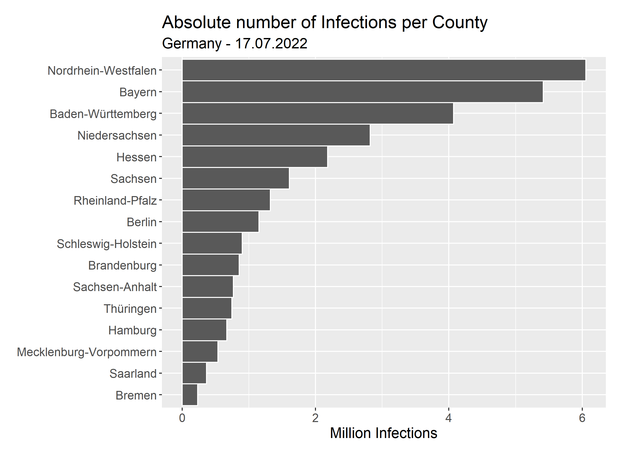
Here, we can see the absolute number of cases per county. This is what we directly extracted without example Pipeline. On its own, the absolute numbers do not tell us a lot, since we have to consider the total population of each county too. So, we download the inhabitants per county from here. Then, we can look at the relative number of infections, which is the number of infections divided by the population per county.
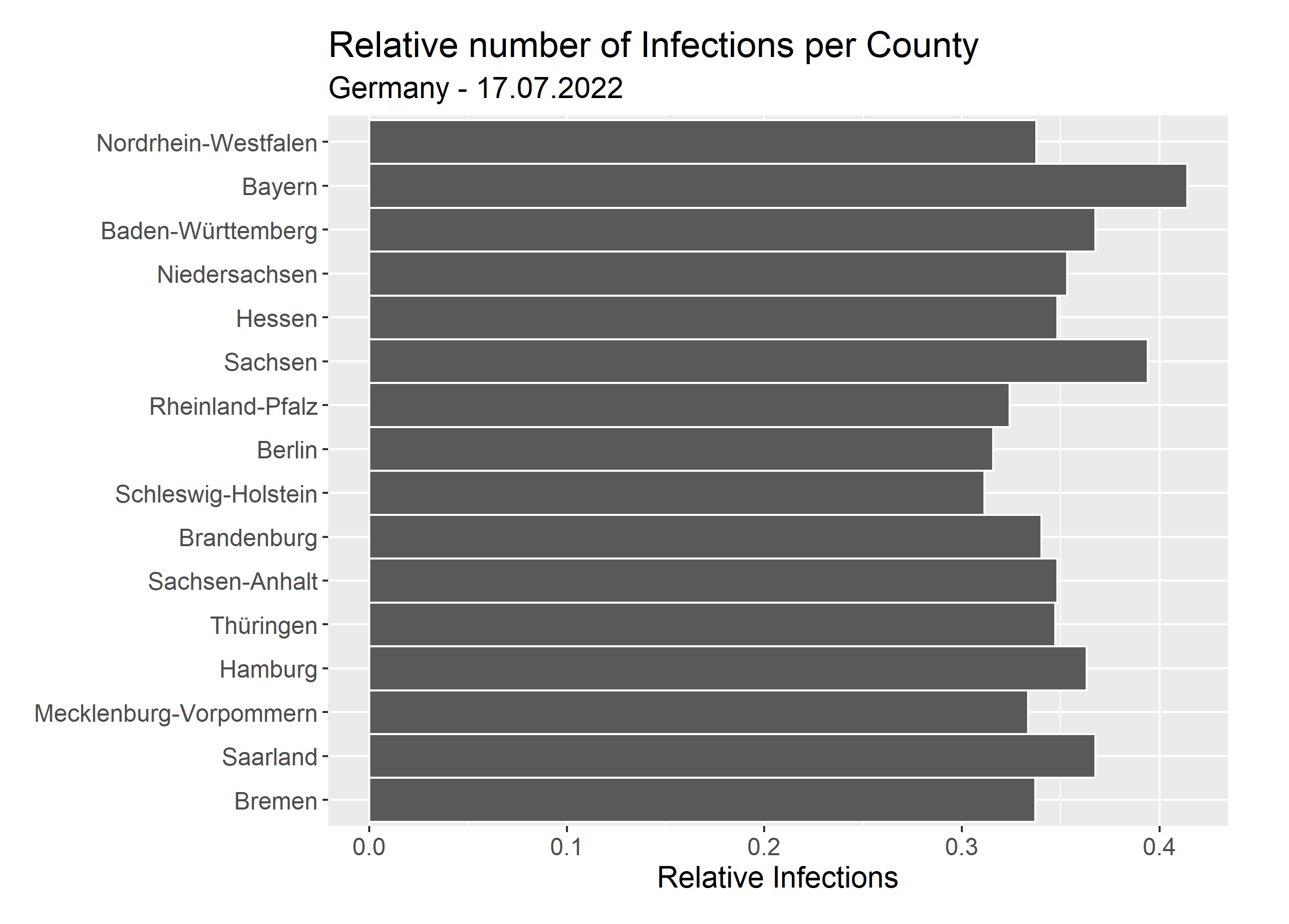
So in contrast to the absolute numbers, we see, that the relative numbers are fairly close to each other. There are many variables to consider when evaluating these numbers: How many tests were made? Were tests available for free? How many people are vaccinated? To do a proper analysis, one would need to dig a lot deeper, but that is not the focus of this article, so we will leave it at this.
Recovered by Agegroup
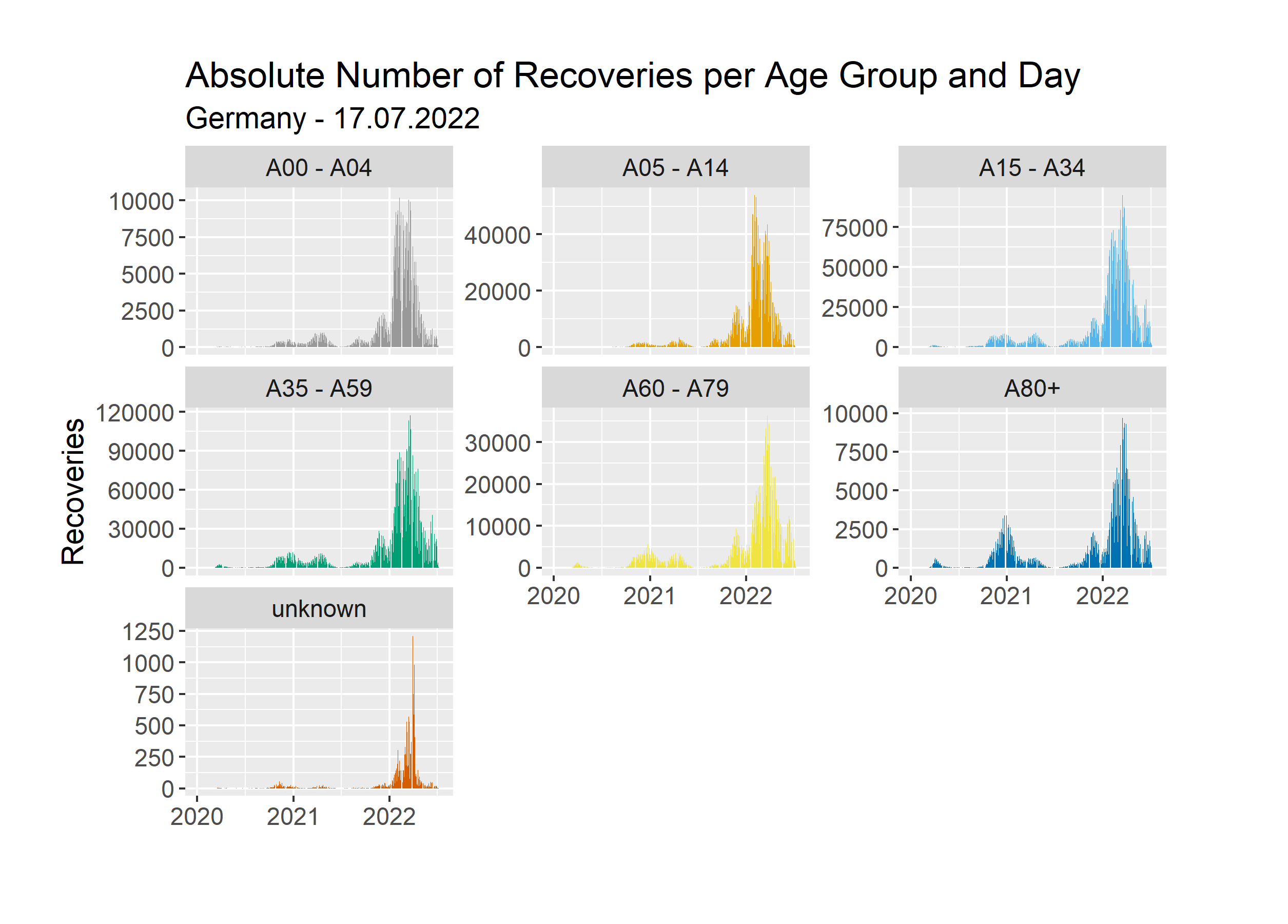
Another Pipeline we created, aggregates the absolute number of recoveries per age group and day. Let’s look at the results.
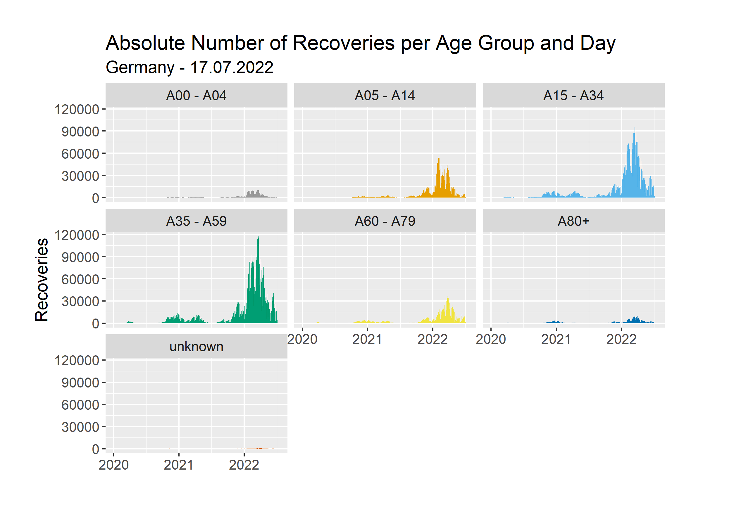
Here we use the same y scale for each age group. We can see, that in absolute numbers the age groups 15-34 and 35-59 stand out. Just like before, this does not consider the total population for each age group. Instead of analyzing that once again, we will look at the same chart with free y scales.
Here we can see if there is any difference in the shape between the graphs for our age groups. We can see, that in general, spikes occur at the same points in time. However, the spikes are not all equally big. Let’s compare the age groups 15-34 and 80+. Both have a big spike during the mid of 2022 and a small one at the start of 2021. If you compare the height of these spikes, you can see, that the spike at the start of 2021 is relatively high for the age group 80+. This could be for a variety of reasons. Perhaps that was the time when people did meet up with their families over Christmas and many infections occurred. The younger people perhaps did not test themselves as much as the elderly people afterwards. Once again, a proper analysis requires more time and data.
Cases by Sex
Another Pipeline aggregates the cases by sex. We represent that in a simple table.
| Sex | Infections |
|---|---|
| Male | 14.184.314 |
| Female | 15.228.545 |
| Unknown | 280.130 |
We see a slightly higher number of cases for females. This could also be due to the fact, that there are more females in Germany than males. The ratio is 50.54% to 49.46% in favor of females. The ratio of cases disregarding unknown ones is 51.77% in favor of females.
Days with most Deaths
The last Pipeline we will look at aggregates the deaths per day and delivers us the 10 days with the most deaths.
| Date | Deaths |
|---|---|
| 2020/12/30 | 1289 |
| 2020/12/23 | 1253 |
| 2020/12/29 | 1249 |
| 2020/12/22 | 1199 |
| 2020/12/17 | 1167 |
| 2020/12/10 | 1078 |
| 2020/12/16 | 1070 |
| 2020/12/18 | 1047 |
| 2021/01/05 | 1041 |
| 2021/01/07 | 1030 |
Most deaths occurred during December of 2020. We see two outliers in May and July of 2021.
Other Pipelines
We had two more Pipelines, which unfortunately were too demanding to run locally with the full dataset. Our first Pipeline determines the difference in infection start and reporting date per county. The second aggregates deaths of persons under the age of 80 per county. Apache Beam is not made for local running, you are only supposed to test it locally on a small dataset. We will omit those here.
Conclusion
Traditionally, we had different systems for different use-cases. Spark for batch-processing. Flink for stream processing. Kafka as a messagebroker. Now, these systems are extended and we can for example do stream-processing in Spark or Kafka. Apache Beam tries to unify these Pipelines since they all operate on a very similar set of operations. While Apache Beam is still relatively new and lacks some features such as removing the header row from a CSV file, it makes distributed Pipelines easy. You can choose from a variety of runners depending on your needs. Check out the available runners and the implemented functionalities here.
Apache Beam is the first framework I have worked with to create distributed data pipelines. The documentation is good and everything is intuitive. I enjoyed working with Apache Beam.